Unit III

Aggregate Demand

• Shows that amount of Real GDP that the private, public, and foreign sectors collectively desire to purchase at each possible price level
• The relationship between the price level and the level of GDP is inverse
• Aggregate Demand (AD) Graph Demand Curve

• Three reasons AD is downward sloping

1. Real-Balances Effect

• When the price-level is high households and businesses cannot afford to purchase as much output
• When the price-level is low households and businesses can afford to purchase output

2. Interest-Rate Effect

• A higher price-level increases the interest rate which tends to discourage investment
• A lower price-level decreases the interest rate which tends to encourage investment

3. Foreign Purchases Effect

• A higher price-level increases the demand for relatively cheaper imports
• A lower price-level increases the foreign demand for relatively cheaper United States imports

• Shifts in AD

-There are two parts to a shift in AD:

1. A change in C, Ig, G, and/or Xn
2. A multiplier effect that produces a greater change than the original change in the 4 components

-Increase in AD=AD shifts to the right

-Decrease in AD=AD shifts to the left

• Consumption

-Household spending is affected by:

1. Consumer wealth

• More wealth=more spending (AD shifts to the right)
• Less wealth=less spending (AD shifts to the left)

2. Consumer expectations

• Positive expectations=more spending (AD shift to the right)
• Negative expectations=less spending (AD shift to the left)

3. Household indebtedness

• Less debt=more spending (AD shifts to the right)
• More debt=less spending (AD shifts to the left)

• Gross Private Investment

-Investment spending is sensitive to:

1. The Real Interest Rate

• Lower=more investment (AD shifts to the right)
• Higher=less investment (AD shifts to the left)

2. Expected Returns

• Higher=more investment (AD shifts to the right)
• Lower=less investment (AD shifts to the left)

3. Expected Returns are influenced by:

• Expectations of future profitability
• Technology
• Degree of excess capacity (existing stock of capital)
• Business taxes

• Government Spending

-More government spending (AD shifts to the right)

-Less government spending (AD shifts to the left)

• Net Exports

-Sensitive to:

• Exchange Rates (international value of dollars)

1. Strong money=more imports and fewer exports (AD shifts to the left)
2. Weak money=fewer imports and more exports (AD shifts to the right)

• Relative Income

1. Strong foreign economies=more exports (AD shifts to the right)
2. Weak foreign economies=less exports (AD shifts to the left)

Aggregate Supply 

• The level of Real (GDPr) that forms will produce at each Price Level (PL)

Long-Run vs. Short-Run 

• Long-Run is a period of time where input prices are completely flexible and adjust to changes in the price-level
• In the long-run, the level of Real GDP supplied is independent of the price-level
• Short-Run is a period of time where input prices are sticky and do not adjust to changes in the price-level
• In the short-run, the level if Real GDP supplied is directly related to the price level

This example shows LRAS and SRAS in the same graph:

Long-Run Aggregate Supply (LRAS)

• The LRAS marks the level of full employment in the economy (analogous to PPC)

Change in the Short-Run

• An increase in SRAS is seen as a shift to right
• A decrease in SRAS is seen as a shift the left
• The key to understanding shifts in SRAS is per unit cost of production 

Per-Unit Production Cost=(total input cost)/(total output)

• Determinants of SRAS

1. Input prices
2. Productivity
3. Legal-institutional environment

• Input Prices

-Domestic Resource Prices

• Wages (75% of all business costs)
• Cost of capital 
• Raw materials (commodity prices)

-Increase in resources prices=SRAS shifts to the right

-Decrease in resource prices=SRAS shifts to the left

• Productivity

Productivity=(total outputs)/(total inputs)

-More productivity=lower unit production cost (SRAS shifts to the right)

-Lower productivity=higher unit production cost (SRAS shifts to the left)

• Legal Productivity

-Tax and Subsidies

• Taxes ($ to government) on business increase per unit production cost (SRAS shifts to the left)
• Subsidies ($ to government) to business reduce per unit production cost (SRAS shifts to the right)

-Government Regulation

• Government regulation creates creates a cost of compliance (SRAS shifts to the left)
• Deregulation reduces compliance cost (SRAS shifts to the right)

The AS/AD Model

• The equilibrium of AS and AD determines current output (GDPr) and the price level (PL)

• Full Employment: full employment equilibrium exists where AD intersect SRAS and LRAS at the same point

• Recessionary Gap: exists when equilibrium occurs below full employment output

• Inflationary Gap: an inflationary gap exists when equilibrium occurs beyond full employment output

\

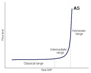
3 Ranges Of The AS Curve

• Horizontal or Keynesian: includes only levels of real output that are less than full employment output, implies that the economy is a recession, therefore you have a decrease in real output
• Vertical or Classical: the economy reaches it's full capacity real output
• Intermediate Range: expansion of real output and price level

Consumption and Saving

• Disposable Income (DI):

-Income after taxes or net income

-Two choices, households can either consume or save

DI=(gross income)-(taxes)

• Consumption:

-Household spending

-The ability to consume is constrained by:

• The amount of disposable income
• The propensity to save
• Autonomous consumption
• Dissaving

APC=C/DI=% DI that is spent

• Saving: 

-Household not spending

-The ability to save is constrained by:

• The amount of disposable income
• The propensity to consume

APS=S/DI=% DI that is not spent

• APC & APS

-APC: average propensity to consume

-APS: average propensity to spend

APC+APS=1

1-APC=APS

1-APS=APC

APC>1: Dissaving 

(-APS):Dissaving

• MPC & MPS

-Marginal Propensity to Consume

-Percent of every extra dollar earned that is spent

MPC=(Change in Consumption)/(Change in Disposable Income) 

-Marginal Propensity to Save

-Percent of every extra dollar earned that is saved

MPC=(Change in Savings)/(Change in Disposable Income)

MPC+MPS=1

1-MPC=MPS

1-MPS=MPC

If you need more help, refer to this!

• Determinants on Consumption and Savings: wealth, expectations, household debt, taxes
• The Spending Multiplier: an initial change in spending causes a larger change in aggregate spending or AD

Multiplier=(Change in AD)/(Change in Spending)

Multiplier=(Change in AD)/(Change in C, G, I, or X)

-Expenditures and income flow continuously which sets off a spending increase in the economy

• Calculating The Spending Multiplier

-Multipliers are (+) when there is an increase in spending and (-) when there is a decrease

• Calculating The Tax Multiplier

-When the government taxes, the multiplier works inverse

-Money is leaving the circular flow

-If there is a tax cut, then the multiplier is positive, because there is now more money in the circular flow

Interest Rate and Investment Demand 

• Investment: money spent or expenditures on

1. New plants (factories)
2. Capital equipment (machinery)
3. Technology (hardware and software)
4. New homes
5. Inventories (goods sold by producers)

• Expected Rates of Return

-How to make decisions: cost/benefit analysis

-How to determine benefits: expected rate of return

-How businesses count the cost: interest costs

-How businesses determine the amount of investment they undertake: compare expected rate of return to interest cost

• If expected return > interest cost, then invest
• If expected return < interest cost, do not invest

• Real (r%) v. Nominal (i%)

-Nominal is the observable rate of interest, real subtracts out inflation an is only know as expost facto

-The real interest rate determines the cost of an investment decision

• Investment Demand Curve (ID)

-Downward sloping

-When interest rates are high, fewer investments are profitable; when interest rates are low, more investments are profitable

-Shifts in ID:

1. Cost of production
2. Business taxes
3. Technological change
4. Stock of capital 
5. Expectations

Fiscal Policy

• Changes in the expenditures or tax revenues of the federal government
• Two tools for fiscal policy:

1. Taxes: government can increase or decrease
2. Spending: government can increase or decrease spending

• Fiscal policy is enacted to promotes our nation's economic goals: full employment, price stability, economic growth
• Deficit, Surpluses, and Debt

Balance Budget: revenues-expenditures

Budget Deficit: revenues<expenditures

Budget Surplus: revenues>expenditures

Government Debt: sum of all deficits-sum of all surpluses

• Government must borrow money when it ruins a budget deficit
• Government borrows from:

1. Individuals
2. Corporations
3. Financial institutions
4. Foreign entities or foreign government

• Two Options (Fiscal Policy)

1. Discretionary (action)

• Expansionary: think deficit
• Contractionary: think surplus

2. Non-Discretionary (non-action)

• Discretionary v. Automatic

-Discretionary: decreasing or increasing tax or spending

-Automatic: unemployment compensation

• Contractionary v. Expansionary

-Contractionary: policy designed to decrease AD, strategy for controlling inflation

-Expansionary: policy designed to increase AD, strategy for increasing GDP combating a recession and reducing unemployment

• Expansionary Fiscal Policy: recession is countered with expansionary policy

-Increase government spending

-Decrease taxes

-Price level increases: this mean expansionary fiscal policy creates some inflation

• Contractionary Fiscal Policy: inflation is countered with contractionary policy

-Decrease government spending 

-Increase taxes 

-U% increased: this means contractionary 

• Automatic or Built in Stabilizer: anything that increases the government budget deficit during a recession and increases it's budget surpluses during inflation without requiring action from policy makers (social security)
• Three Taxes Systems

1. Progressive Tax System: average tax rate that rises with GDP
2. Proportional Tax System: average tax rate remains constant as GDP changes
3. Regressive Tax System: average tax rate falls with GDP