Unit IV (Chapter 13&14)

Chapter 13

Uses of Money 

1. Medium Exchange: using to barter our trade
2. Unit of Account: gives money economic worth
3. Store of Value: dollar does not fluctuate

Types of Money

1. Representative Money: paper money that is backed by a tangible product
2. Commodity Money: gold a silver coins, gets value from material that is is made of 
3. Flat Money: money because government said so 

Characteristics of money 

1. Durability: 
2. Portability: carry money everywhere
3. Divisibility: money can be broken down
4. Uniformity: money is identical
5. Scarcity:
6. Acceptability: 

M1 Money (more liquid) 

• Consist of currency circulation (paper and coins)
• Travelers checks
• Checkable deposits
• Demand deposits

M2 Money 

• Savings accounts
• Money market accounts
• Accounts held by banks outside of the United States
• Adding M1 money

Chapter 14

• Assets=(Liabilities)+(Net Worth) 
• Reserve Ration=(Commercial Bank's Required Reserves)/(Commercial Bank's Checkable Deposit Liabilities)

Three Important Issues

1. Excess Reserves=(Actual Reserves)-(Required Reserves)
2. Control of lending liability
3. Asset or liability to which bank?

• Banks create money by lending excess reserves and destroy it by loan payment , purchasing bonds from the public also creates money
• Money Multiplier=(1)/(Required Reserve Ratio)
• Maximum Checkable Deposit Creation=(Excess Reserves)(Monetary Multiplier)

Mr. Mac AP Macroeconomics-Multiple Deposit Expansion

Reserve Equipment 

• The Fed requires banks to always have some money readily available to meet consumers' demand for cash
• The amount, set by the Fed, is the required reserve ratio
• The required reserve ratio is the percentage of demand deposits (checking account balance) that must not be loaned out
• Typically the required reserve ration equals 10%

The Money Multiplier

• Similar to the spending multiplier, the money multiplier shows us the impact of a change in demand deposits on loans and eventually the money supply
• To calculate the multiplier, divide 1 by the required reverse ratio
• Money Multiplier=(1)/(Reserve Ratio)

The Three Types of Multiplier of Multiple Deposit Expansion

Type 1

• Calculate the initial change in excess reserves
• The smount of a single bank can loan from the initial deposit

Type 2

• Calculate the change in loans in the banking system

Type 3

• Calculate the change in the money supply
• Sometimes type 2 and 3 will have the same result (no Fed involvement)

Monetary Policy (Federal Reserve Bank)

• Influencing the economy through changes in reserves which influences the money supply and available credit

4 Options of Monetary Policy

1. Reserve Requirement: percent that is set by the FED of the minimum reserve a bank must keep
2. Discount Rate: the rate of interest that the FED charges for overnight loans to banks
3. Federal Fund Rate: rate that FDIC members charge each other for loans 
4. OMO (Open Market Operation): either buy or sell securities (bonds)

• If the FED buys bonds they expand (expansionary) money supply
• If they sell bonds they decrease money supply (contractionary)

Prime Rate

• Interest rate that banks charge their most credit worthy borrowers

	Expansionary	Contractionary
OMO	Buy Bonds	Sell Bonds
Discount Rate	↓	↑
Federal Fund Rate	↓	↑
Required Reserve Ratio	↓	↑

• If initial deposit is not new money, the total change in money supply is only the new money created by the banking system
• Single Bank: amount of money single banks can create (loan out)=ER

AR-RR+ER

• Banking Sytem: can create money by a multiple of its initial ER

Deposit Multiplier= (1)/(RR)

System New Money= (Deposit Multiplier)(Initial ER)

To understand the unit better, watch this!

Graphs that might help understand Monetary Policy more!

Money & Banking/ Monetary Supply Video Notes

Unit 4- Part 1

There are three types of money; commodity, representative, and FIAT. Commodity represents good that can also be represented as money. Representative money which is money backed up by gold, and FIAT being the opposite of that. There are also three functions of money; medium of exchange, store of value, and unit of account. Medium of exchange is a substances through which things pass. Store value meaning that you still want money that you could be possibly saving to keep its value, you want it to be worth just as much later. Unit of account deals how price equals worth/value.
This was the information that I was able to learn when watching the video. It was extremely helpful when getting the basic understanding of the types of money and what each one of them actually means. The video was also not complicated to understand too.

Unit 4- Part 3

The price that you pay to get money is the interest rate, meaning that the interest rate would be on your vertical axis. Along your vertical axis you put quantity money on your horizontal axis. The demand of money always slopes down because when the price is high, quantity demanded is low. When the interest rate is low people want to borrow money more. Transaction demand and asset demand are the component of the demand of money. Supply of money is vertical because it does not vary on the interest rate. When increasing demand (shifting left), pressure is put on interest rate causing it to rise; the quantity stays the same because supply of money is vertical. In order to stabilize interest rates, the supply of money must shift to the right.
This video was extremely simple and something that I have already sort of seen before. It went over basic understandings of which there is a slope with the demand of money and the vertical line of supply of money. I found the video extremely helpful.

Unit 4- Part 4

There are three tools of monetary policy that the Fed has; two of these are expansionary and contractionary. If the Fed wants to expand money supply they decrease the required reserves and if they want to contract they would increase the required reserves. If they decrease the required reserves there will be more excess reserves to use on loans. If the Fed wants banks to borrow more money they would lower the discount rate, and if they want to discourage banks they raise the discount rate. To increase money supply the Fed would buy bonds, and to contract the money supply they would sell bonds. The Federal Open Market Committee makes the decisions. The Federal Funds Rate is the rate at which banks borrow money from each; it has nothing to do with the Fed.
This video went expansionary and contractionary dealing with monetary policy. It was something I had already learned before in the previous unit, but the video gave me a more clearer understanding of it and its use in this unit.

Unit 4- Part 7

I found it really hard to retain information from this video. The lady did not explain everything clearly and the work she did on the smart board became confusing after a period of time. I did not find the video as helpful as the previous ones.

Unit 4- Part 8

The video was a review of the work we had been doing in class, it was simple to understand as well.The video was a review of how to find the multiplier and how you apply the required reserve to the problem, specifically to the loans.

Unit 4-Part 9

I found this video hard to understand. The explanations did not really make sense to me. The information videos seem to be the ones that do not have to do with the money demand graphs. I did not find the video very helpful.

Unit III

Aggregate Demand

• Shows that amount of Real GDP that the private, public, and foreign sectors collectively desire to purchase at each possible price level
• The relationship between the price level and the level of GDP is inverse
• Aggregate Demand (AD) Graph Demand Curve

• Three reasons AD is downward sloping

1. Real-Balances Effect

• When the price-level is high households and businesses cannot afford to purchase as much output
• When the price-level is low households and businesses can afford to purchase output

2. Interest-Rate Effect

• A higher price-level increases the interest rate which tends to discourage investment
• A lower price-level decreases the interest rate which tends to encourage investment

3. Foreign Purchases Effect

• A higher price-level increases the demand for relatively cheaper imports
• A lower price-level increases the foreign demand for relatively cheaper United States imports

• Shifts in AD

-There are two parts to a shift in AD:

1. A change in C, Ig, G, and/or Xn
2. A multiplier effect that produces a greater change than the original change in the 4 components

-Increase in AD=AD shifts to the right

-Decrease in AD=AD shifts to the left

• Consumption

-Household spending is affected by:

1. Consumer wealth

• More wealth=more spending (AD shifts to the right)
• Less wealth=less spending (AD shifts to the left)

2. Consumer expectations

• Positive expectations=more spending (AD shift to the right)
• Negative expectations=less spending (AD shift to the left)

3. Household indebtedness

• Less debt=more spending (AD shifts to the right)
• More debt=less spending (AD shifts to the left)

• Gross Private Investment

-Investment spending is sensitive to:

1. The Real Interest Rate

• Lower=more investment (AD shifts to the right)
• Higher=less investment (AD shifts to the left)

2. Expected Returns

• Higher=more investment (AD shifts to the right)
• Lower=less investment (AD shifts to the left)

3. Expected Returns are influenced by:

• Expectations of future profitability
• Technology
• Degree of excess capacity (existing stock of capital)
• Business taxes

• Government Spending

-More government spending (AD shifts to the right)

-Less government spending (AD shifts to the left)

• Net Exports

-Sensitive to:

• Exchange Rates (international value of dollars)

1. Strong money=more imports and fewer exports (AD shifts to the left)
2. Weak money=fewer imports and more exports (AD shifts to the right)

• Relative Income

1. Strong foreign economies=more exports (AD shifts to the right)
2. Weak foreign economies=less exports (AD shifts to the left)

Aggregate Supply 

• The level of Real (GDPr) that forms will produce at each Price Level (PL)

Long-Run vs. Short-Run 

• Long-Run is a period of time where input prices are completely flexible and adjust to changes in the price-level
• In the long-run, the level of Real GDP supplied is independent of the price-level
• Short-Run is a period of time where input prices are sticky and do not adjust to changes in the price-level
• In the short-run, the level if Real GDP supplied is directly related to the price level

This example shows LRAS and SRAS in the same graph:

Long-Run Aggregate Supply (LRAS)

• The LRAS marks the level of full employment in the economy (analogous to PPC)

Change in the Short-Run

• An increase in SRAS is seen as a shift to right
• A decrease in SRAS is seen as a shift the left
• The key to understanding shifts in SRAS is per unit cost of production 

Per-Unit Production Cost=(total input cost)/(total output)

• Determinants of SRAS

1. Input prices
2. Productivity
3. Legal-institutional environment

• Input Prices

-Domestic Resource Prices

• Wages (75% of all business costs)
• Cost of capital 
• Raw materials (commodity prices)

-Increase in resources prices=SRAS shifts to the right

-Decrease in resource prices=SRAS shifts to the left

• Productivity

Productivity=(total outputs)/(total inputs)

-More productivity=lower unit production cost (SRAS shifts to the right)

-Lower productivity=higher unit production cost (SRAS shifts to the left)

• Legal Productivity

-Tax and Subsidies

• Taxes ($ to government) on business increase per unit production cost (SRAS shifts to the left)
• Subsidies ($ to government) to business reduce per unit production cost (SRAS shifts to the right)

-Government Regulation

• Government regulation creates creates a cost of compliance (SRAS shifts to the left)
• Deregulation reduces compliance cost (SRAS shifts to the right)

The AS/AD Model

• The equilibrium of AS and AD determines current output (GDPr) and the price level (PL)

• Full Employment: full employment equilibrium exists where AD intersect SRAS and LRAS at the same point

• Recessionary Gap: exists when equilibrium occurs below full employment output

• Inflationary Gap: an inflationary gap exists when equilibrium occurs beyond full employment output

\

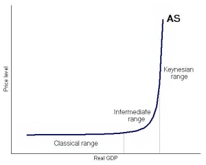
3 Ranges Of The AS Curve

• Horizontal or Keynesian: includes only levels of real output that are less than full employment output, implies that the economy is a recession, therefore you have a decrease in real output
• Vertical or Classical: the economy reaches it's full capacity real output
• Intermediate Range: expansion of real output and price level

Consumption and Saving

• Disposable Income (DI):

-Income after taxes or net income

-Two choices, households can either consume or save

DI=(gross income)-(taxes)

• Consumption:

-Household spending

-The ability to consume is constrained by:

• The amount of disposable income
• The propensity to save
• Autonomous consumption
• Dissaving

APC=C/DI=% DI that is spent

• Saving: 

-Household not spending

-The ability to save is constrained by:

• The amount of disposable income
• The propensity to consume

APS=S/DI=% DI that is not spent

• APC & APS

-APC: average propensity to consume

-APS: average propensity to spend

APC+APS=1

1-APC=APS

1-APS=APC

APC>1: Dissaving 

(-APS):Dissaving

• MPC & MPS

-Marginal Propensity to Consume

-Percent of every extra dollar earned that is spent

MPC=(Change in Consumption)/(Change in Disposable Income) 

-Marginal Propensity to Save

-Percent of every extra dollar earned that is saved

MPC=(Change in Savings)/(Change in Disposable Income)

MPC+MPS=1

1-MPC=MPS

1-MPS=MPC

If you need more help, refer to this!

• Determinants on Consumption and Savings: wealth, expectations, household debt, taxes
• The Spending Multiplier: an initial change in spending causes a larger change in aggregate spending or AD

Multiplier=(Change in AD)/(Change in Spending)

Multiplier=(Change in AD)/(Change in C, G, I, or X)

-Expenditures and income flow continuously which sets off a spending increase in the economy

• Calculating The Spending Multiplier

-Multipliers are (+) when there is an increase in spending and (-) when there is a decrease

• Calculating The Tax Multiplier

-When the government taxes, the multiplier works inverse

-Money is leaving the circular flow

-If there is a tax cut, then the multiplier is positive, because there is now more money in the circular flow

Interest Rate and Investment Demand 

• Investment: money spent or expenditures on

1. New plants (factories)
2. Capital equipment (machinery)
3. Technology (hardware and software)
4. New homes
5. Inventories (goods sold by producers)

• Expected Rates of Return

-How to make decisions: cost/benefit analysis

-How to determine benefits: expected rate of return

-How businesses count the cost: interest costs

-How businesses determine the amount of investment they undertake: compare expected rate of return to interest cost

• If expected return > interest cost, then invest
• If expected return < interest cost, do not invest

• Real (r%) v. Nominal (i%)

-Nominal is the observable rate of interest, real subtracts out inflation an is only know as expost facto

-The real interest rate determines the cost of an investment decision

• Investment Demand Curve (ID)

-Downward sloping

-When interest rates are high, fewer investments are profitable; when interest rates are low, more investments are profitable

-Shifts in ID:

1. Cost of production
2. Business taxes
3. Technological change
4. Stock of capital 
5. Expectations

Fiscal Policy

• Changes in the expenditures or tax revenues of the federal government
• Two tools for fiscal policy:

1. Taxes: government can increase or decrease
2. Spending: government can increase or decrease spending

• Fiscal policy is enacted to promotes our nation's economic goals: full employment, price stability, economic growth
• Deficit, Surpluses, and Debt

Balance Budget: revenues-expenditures

Budget Deficit: revenues<expenditures

Budget Surplus: revenues>expenditures

Government Debt: sum of all deficits-sum of all surpluses

• Government must borrow money when it ruins a budget deficit
• Government borrows from:

1. Individuals
2. Corporations
3. Financial institutions
4. Foreign entities or foreign government

• Two Options (Fiscal Policy)

1. Discretionary (action)

• Expansionary: think deficit
• Contractionary: think surplus

2. Non-Discretionary (non-action)

• Discretionary v. Automatic

-Discretionary: decreasing or increasing tax or spending

-Automatic: unemployment compensation

• Contractionary v. Expansionary

-Contractionary: policy designed to decrease AD, strategy for controlling inflation

-Expansionary: policy designed to increase AD, strategy for increasing GDP combating a recession and reducing unemployment

• Expansionary Fiscal Policy: recession is countered with expansionary policy

-Increase government spending

-Decrease taxes

-Price level increases: this mean expansionary fiscal policy creates some inflation

• Contractionary Fiscal Policy: inflation is countered with contractionary policy

-Decrease government spending 

-Increase taxes 

-U% increased: this means contractionary 

• Automatic or Built in Stabilizer: anything that increases the government budget deficit during a recession and increases it's budget surpluses during inflation without requiring action from policy makers (social security)
• Three Taxes Systems

1. Progressive Tax System: average tax rate that rises with GDP
2. Proportional Tax System: average tax rate remains constant as GDP changes
3. Regressive Tax System: average tax rate falls with GDP